Version information
[1]:
%matplotlib notebook
from PySide2.QtWidgets import *
from datetime import date
print("Running date: ", date.today().strftime("%B %d, %Y"))
import pyleecan
print("Pyleecan version: " + pyleecan.__version__)
import SciDataTool
print("SciDataTool version: " + SciDataTool.__version__)
Running date:  April 27, 2023
Pyleecan version: 1.5.0
SciDataTool version: 2.5.0
How to define a machine
This tutorial shows the different ways to define electrical machine. To do so, it presents the definition of the Toyota Prius 2004 interior magnet with distributed winding [1].
The notebook related to this tutorial is available on GitHub.
Type of machines Pyleecan can model
The architecture of Pyleecan also enables to define other kinds of machines (with more than two laminations for instance). More information in our ICEM 2020 pyblication [2]
Every machine can be defined by using the Graphical User Interface or directly in Python script.
Defining machine with Pyleecan GUI
Each parameter is explained by a tooltip and the machine can be previewed at each stage of the design.
Start the GUI
The GUI can be started by running the following command in a notebook:
# Start Pyleecan GUI from the Jupyter Notebook
%run -m pyleecan
To use it on Anaconda you may need to create the system variable:
QT_QPA_PLATFORM_PLUGIN_PATH : path:nbsphinx-math:to\anaconda3\Lib\site-packages:nbsphinx-math:PySide2\plugins\platforms
The GUI can also be launched in command line/terminal by calling one of the following commands in a terminal:
Path/to/python.exe -m pyleecan
Path/to/python3.exe -m pyleecan
[2]:
%run -m pyleecan
load a machine
Once the machine defined in the GUI it can be loaded and plot with the following commands:
[3]:
%matplotlib inline

# Load the machine
from os.path import join
from pyleecan.Functions.load import load
from pyleecan.definitions import DATA_DIR

IPMSM_A = load(join(DATA_DIR, "Machine", "Toyota_Prius.json"))
# In Jupyter notebook, we set is_show_fig=False to skip call to fig.show() to avoid a warning message
# All plot methods return the corresponding matplotlib figure and axis to further edit the resulting plot
fig, ax = IPMSM_A.plot(is_show_fig=False)

Defining Machine in scripting mode
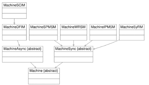
Pyleecan also enables to define the machine in scripting mode, using different classes. Each class is defined from a csv file in the folder pyleecan/Generator/ClasseRef and the documentation of every class is available on the dedicated webpage. The following image shows the machine classes organization :
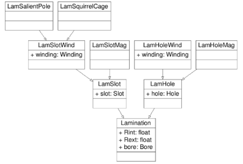
Every rotor and stator can be created with the Lamination class or one of its daughters.
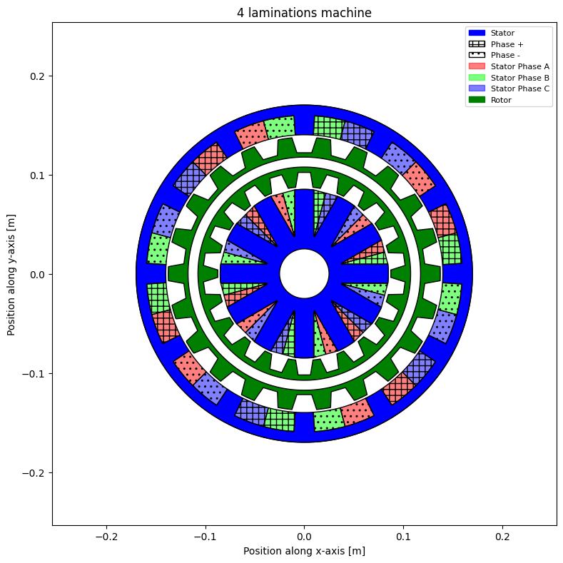
The scripting enables to define some complex and exotic machine that can’t be defined in the GUI such as this one:
[4]:
from pyleecan.Classes.MachineUD import MachineUD
from pyleecan.Classes.LamSlotWind import LamSlotWind
from pyleecan.Classes.LamSlot import LamSlot
from pyleecan.Classes.Winding import Winding
from pyleecan.Classes.SlotW10 import SlotW10
from pyleecan.Classes.SlotW22 import SlotW22
from numpy import pi

machine = MachineUD(name="4 laminations machine", shaft=None)

# Main geometry parameter
Rext = 170e-3  # Exterior radius of outter lamination
W1 = 30e-3  # Width of first lamination
A1 = 2.5e-3  # Width of the first airgap
W2 = 20e-3
A2 = 10e-3
W3 = 20e-3
A3 = 2.5e-3
W4 = 60e-3

# Outer stator
lam1 = LamSlotWind(Rext=Rext, Rint=Rext - W1, is_internal=False, is_stator=True)
lam1.slot = SlotW22(
    Zs=12, W0=2 * pi / 12 * 0.75, W2=2 * pi / 12 * 0.75, H0=0, H2=W1 * 0.65
)
lam1.winding = Winding(qs=3, p=2, Nlayer=2)
# External Rotor
lam2 = LamSlot(
    Rext=lam1.Rint - A1, Rint=lam1.Rint - A1 - W2, is_internal=True, is_stator=False
)
lam2.slot = SlotW10(Zs=22, W0=25e-3, W1=25e-3, W2=15e-3, H0=0, H1=0, H2=W2 * 0.75)
# Internal Rotor
lam3 = LamSlot(
    Rext=lam2.Rint - A2,
    Rint=lam2.Rint - A2 - W3,
    is_internal=False,
    is_stator=False,
)
lam3.slot = SlotW10(
    Zs=22, W0=17.5e-3, W1=17.5e-3, W2=12.5e-3, H0=0, H1=0, H2=W3 * 0.75
)
# Inner stator
lam4 = LamSlotWind(
    Rext=lam3.Rint - A3, Rint=lam3.Rint - A3 - W4, is_internal=True, is_stator=True
)
lam4.slot = SlotW10(Zs=12, W0=25e-3, W1=25e-3, W2=1e-3, H0=0, H1=0, H2=W4 * 0.75)
lam4.winding = Winding(qs=3, p=2, Nlayer=2)
# Machine definition
machine.lam_list = [lam1, lam2, lam3, lam4]

# Plot, check and save
fig, ax = machine.plot(is_show_fig=False)
Stator definition
To define the stator, we initialize a LamSlotWind object (a Lamination with Slot containing Winding) with the different parameters. In pyleecan, all the parameters must be set in SI units.
[5]:
from pyleecan.Classes.LamSlotWind import LamSlotWind
mm = 1e-3  # Millimeter


# Lamination setup
stator = LamSlotWind(
    Rint=80.95 * mm, # internal radius [m]
    Rext=134.62 * mm, # external radius [m]
    L1=83.82 * mm, # Lamination stack active length [m] without radial ventilation airducts
                # but including insulation layers between lamination sheets
    Nrvd=0, # Number of radial air ventilation duct
    Kf1=0.95, # Lamination stacking / packing factor
    is_internal=False,
    is_stator=True,
)
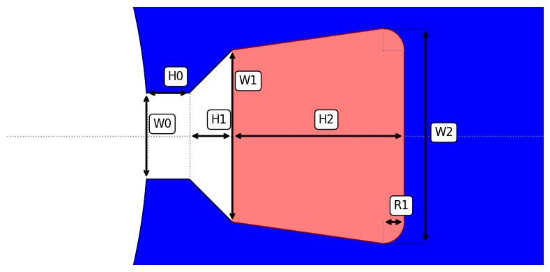
Then we add 48 slots using SlotW11 which is one of the 25 Slot classes. All the schematics are available in the GUI, on Github or with the “plot_schematics” method:
[6]:
from pyleecan.Classes.SlotW11 import SlotW11

# Slot setup
stator.slot = SlotW11(
    Zs=48, # Slot number
    H0=1.0 * mm,  # Slot isthmus height
    H1=0, # Height
    H2=33.3 * mm, # Slot height below wedge
    W0=1.93 * mm,  # Slot isthmus width
    W1=5 * mm, # Slot top width
    W2=8 * mm, # Slot bottom width
    R1=4 * mm # Slot bottom radius
)
fig, ax = stator.slot.plot_schematics(is_default=True, is_show_fig=False)
fig, ax = stator.slot.plot(is_show_fig=False)
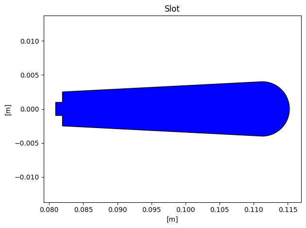
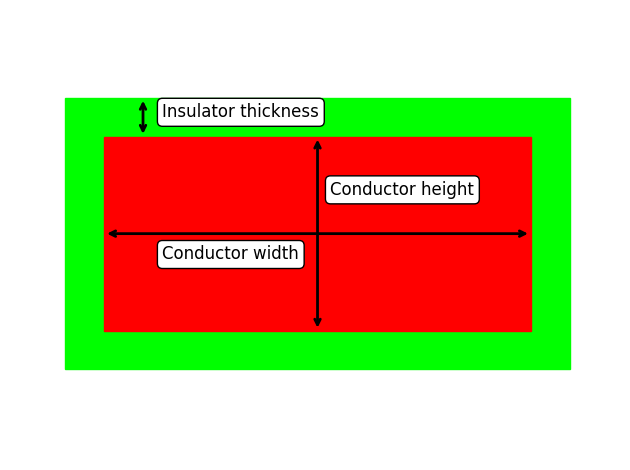
As for the slot, we can define the winding and its conductor with Winding and CondType11 (CondType11 is Form wound / rectangular wire). The conventions for winding are further explained on pyleecan website
[7]:
from pyleecan.Classes.Winding import Winding
from pyleecan.Classes.CondType11 import CondType11
# Winding setup
stator.winding = Winding(
    qs=3,  # number of phases
    p=4,  # number of pole pairs
    Nlayer=1,  # Number of layers per slots
    coil_pitch=0, # Coil pitch (or coil span or Throw)
    Lewout=0,  # staight length of conductor outside lamination before EW-bend
    Ntcoil=9,  # number of turns per coil
    Npcp=1,  # number of parallel circuits per phase
    Nslot_shift_wind=0,  # 0 not to change the stator winding connection matrix built by pyleecan number
                         # of slots to shift the coils obtained with pyleecan winding algorithm
                         # (a, b, c becomes b, c, a with Nslot_shift_wind1=1)
    is_reverse_wind=False # True to reverse the default winding algorithm along the airgap
                         # (c, b, a instead of a, b, c along the trigonometric direction)
)

# Conductor setup
stator.winding.conductor = CondType11(
    Nwppc_tan=1, # stator winding number of preformed wires (strands)
                 # in parallel per coil along tangential (horizontal) direction
    Nwppc_rad=1, # stator winding number of preformed wires (strands)
                 # in parallel per coil along radial (vertical) direction
    Wwire=0.000912, #  single wire width without insulation [m]
    Hwire=2e-3, # single wire height without insulation [m]
    Wins_wire=1e-6, # winding strand insulation thickness [m]
    type_winding_shape=0, # type of winding shape for end winding length calculation
                          # 0 for hairpin windings
                          # 1 for normal windings
)
print("Nwppc_rad=Nwppc_tan=1")
fig, ax = stator.winding.conductor.plot_schematics(is_default=True, is_single=True, is_show_fig=False)
Nwppc_rad=Nwppc_tan=1
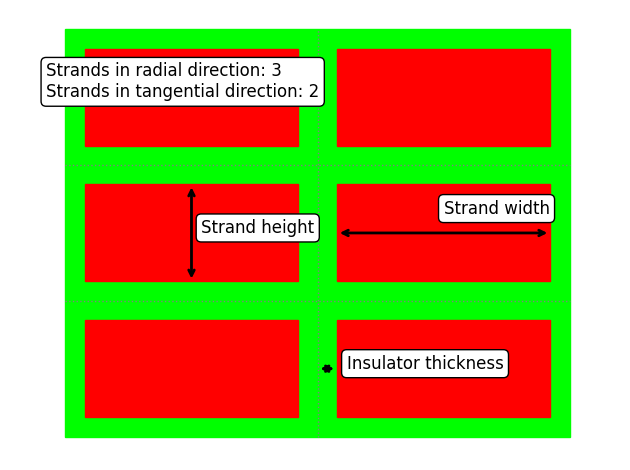
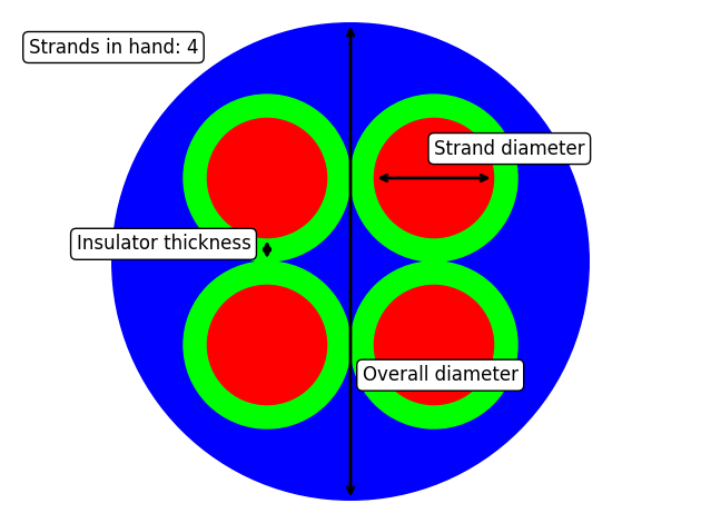
Another schematics is available with more than one strands:
[8]:
print("More than one strands")
fig, ax = stator.winding.conductor.plot_schematics(is_default=True, is_single=False, is_show_fig=False)
More than one strands
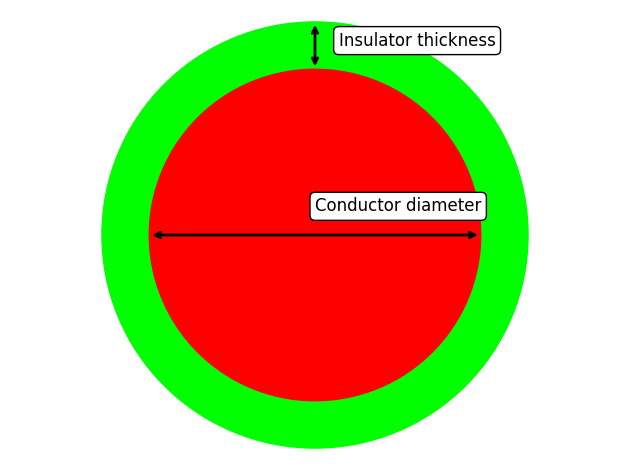
Stranded coil are also available by using a CondType12 object.
[9]:
from pyleecan.Classes.CondType12 import CondType12

cond = CondType12()
fig, ax = cond.plot_schematics(is_default=True, is_single=True, is_show_fig=False)
fig, ax = cond.plot_schematics(is_default=True, is_single=False, is_show_fig=False)
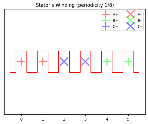
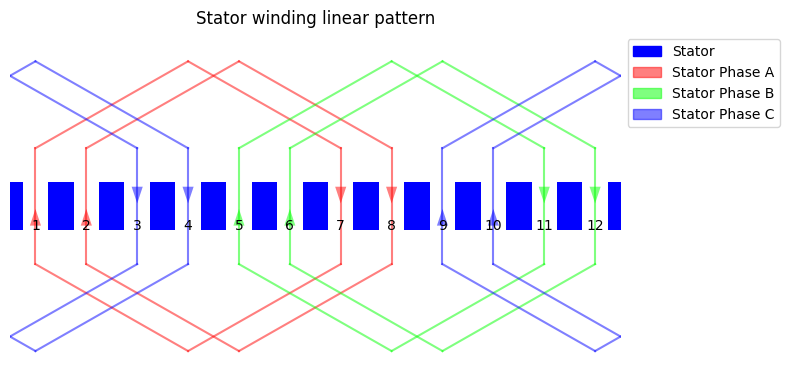
The winding pattern is defined with the star of slot method (thanks to swat-em package) according to Zs, qs, p, Nlayer and coil_pitch.
[10]:
stator.winding.comp_connection_mat()  # Compute the winding pattern with swat-em
wind_mat = stator.winding.get_connection_mat()
# The resulting winding matrix is:
# 1 rad layer, 1 tan layer, 48 slots, 3 phases
print(wind_mat.shape)
print(wind_mat)
(1, 1, 48, 3)
[[[[ 9.  0.  0.]
   [ 9.  0.  0.]
   [ 0.  0. -9.]
   [ 0.  0. -9.]
   [ 0.  9.  0.]
   [ 0.  9.  0.]
   [-9.  0.  0.]
   [-9.  0.  0.]
   [ 0.  0.  9.]
   [ 0.  0.  9.]
   [ 0. -9.  0.]
   [ 0. -9.  0.]
   [ 9.  0.  0.]
   [ 9.  0.  0.]
   [ 0.  0. -9.]
   [ 0.  0. -9.]
   [ 0.  9.  0.]
   [ 0.  9.  0.]
   [-9.  0.  0.]
   [-9.  0.  0.]
   [ 0.  0.  9.]
   [ 0.  0.  9.]
   [ 0. -9.  0.]
   [ 0. -9.  0.]
   [ 9.  0.  0.]
   [ 9.  0.  0.]
   [ 0.  0. -9.]
   [ 0.  0. -9.]
   [ 0.  9.  0.]
   [ 0.  9.  0.]
   [-9.  0.  0.]
   [-9.  0.  0.]
   [ 0.  0.  9.]
   [ 0.  0.  9.]
   [ 0. -9.  0.]
   [ 0. -9.  0.]
   [ 9.  0.  0.]
   [ 9.  0.  0.]
   [ 0.  0. -9.]
   [ 0.  0. -9.]
   [ 0.  9.  0.]
   [ 0.  9.  0.]
   [-9.  0.  0.]
   [-9.  0.  0.]
   [ 0.  0.  9.]
   [ 0.  0.  9.]
   [ 0. -9.  0.]
   [ 0. -9.  0.]]]]
[11]:
fig, ax = stator.plot_winding(is_show_fig=False)   # Show winding pattern smallest sym
fig, ax = stator.winding.plot_linear(is_show_fig=False)
[12]:
fig, ax = stator.plot(
                is_winding_connection=True,
                is_show_fig=False,
                is_add_sign=True,
            )
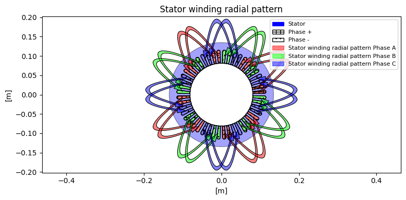
To go further with winding: - WindingUD enables to manually define the winding pattern by enforcing the connexion matrix with the wind_mat property. - SlotUD2 enables to create user-defined winding layer geometry.
Examples can be found in the our ICEM 2020 pyblication [2] (corresponding code available in fig 16 & 17 in https://github.com/Eomys/pyleecan/blob/master/Tests/Plot/test_ICEM_2020.py)
Rotor definition
For this example, we use the LamHole class (a Lamination with Hole/pockets) to define the rotor. The same object is used to define the rotor for SynRM machines by defining a Hole without magnet.
In the same way as for the stator, we start by defining the lamination:
[13]:
from pyleecan.Classes.LamHole import LamHole

# Rotor setup
rotor = LamHole(
    Rint=55.32 * mm, # Internal radius
    Rext=80.2 * mm, # external radius
    is_internal=True,
    is_stator=False,
    L1=stator.L1 # Lamination stack active length [m]
                 # without radial ventilation airducts but including insulation layers between lamination sheets
)
After that, we can add holes with magnets to the rotor using the class HoleM50:
[14]:
from pyleecan.Classes.HoleM50 import HoleM50
rotor.hole = list()
rotor.hole.append(
    HoleM50(
        Zh=8, # Number of Hole around the circumference
        W0=42.0 * mm,  # Slot opening
        W1=0, # Tooth width (at V bottom)
        W2=0, # Distance Magnet to bottom of the V
        W3=14.0 * mm, # Tooth width (at V top)
        W4=18.9 * mm, # Magnet Width
        H0=10.96 * mm, # Slot Depth
        H1=1.5 * mm, # Distance from the lamination Bore
        H2=1 * mm, # Additional depth for the magnet
        H3=6.5 * mm, # Magnet Height
        H4=0, # Slot top height
    )
)
fig, ax = rotor.hole[0].plot_schematics(is_default=True, is_show_fig=False)
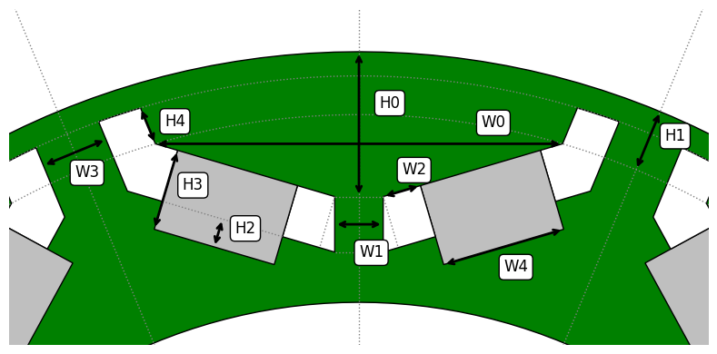
The holes are defined as a list to enable to create several layers of holes and/or to combine different kinds of holes
Create a shaft and a frame
The classes Shaft and Frame enable to add a shaft and a frame to the machine. For this example there is no frame so the object is set as None (corresponding code is there as a exemple):
[15]:
from pyleecan.Classes.Shaft import Shaft
from pyleecan.Classes.Frame import Frame

# Set shaft
shaft = Shaft(Drsh=rotor.Rint * 2, # Diamater of the rotor shaft [m]
                                   # used to estimate bearing diameter for friction losses
              Lshaft=1.2 # length of the rotor shaft [m]
             )
frame = None
#frame = Frame(Rint=stator.Rext, Rext=stator.Rext+0.02, Lfra=stator.L1, mat_type=stator.mat_type)
Set materials and magnets
Every Pyleecan object can be saved in JSON using the method save and can be loaded with the load function. In this example, the materials M400_50A and Copper1 are loaded and set in the corresponding properties.
[16]:
# Loading Materials
M400_50A = load(join(DATA_DIR, "Material", "M400-50A.json"))
Copper1 = load(join(DATA_DIR, "Material", "Copper1.json"))

# Set Materials
stator.mat_type = M400_50A  # Stator Lamination material
rotor.mat_type = M400_50A  # Rotor Lamination material
stator.winding.conductor.cond_mat = Copper1  # Stator winding conductor material
A material can also be defined in scripting as any other Pyleecan object. The material Magnet_prius is created with the classes Material and MatMagnetics.
[17]:
from pyleecan.Classes.Material import Material
from pyleecan.Classes.MatMagnetics import MatMagnetics

# Defining magnets
Magnet_prius = Material(name="Magnet_prius")

# Definition of the magnetic properties of the material
Magnet_prius.mag = MatMagnetics(
    mur_lin = 1.05, # Relative magnetic permeability
    alpha_Br = -0.001, # temperature coefficient for remanent flux density /°C compared to 20°C
    Brm20 = 1.24, # magnet remanence induction at 20°C [T]
    Wlam = 0, # lamination sheet width without insulation [m] (0 == not laminated)
)

# Definition of the electric properties of the material
Magnet_prius.elec.rho = 1.6e-06 # Resistivity at 20°C

# Definition of the structural properties of the material
Magnet_prius.struct.rho = 7500.0 # mass per unit volume [kg/m3]
The magnet materials are set with the “magnet_X” property. Pyleecan enables to define different magnetization or material for each magnets of the holes. Here both magnets are defined identical.
[18]:
# Set magnets in the rotor hole
rotor.hole[0].magnet_0.mat_type = Magnet_prius
rotor.hole[0].magnet_1.mat_type = Magnet_prius
rotor.hole[0].magnet_0.type_magnetization = 1
rotor.hole[0].magnet_1.type_magnetization = 1
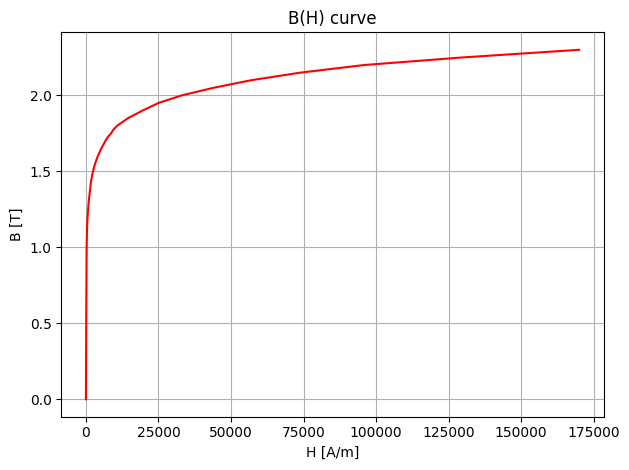
The B(H) curve of any material can be set as a two columns matrix with:
[19]:
BH = [
    [0.0,0.0],
    [100.0,0.5],
    [150.0,0.7],
    [180.0,0.8],
    [200.0,0.9],
    [250.0,1.0],
    [300.0,1.05],
    [350.0,1.1],
    [450.0,1.15],
    [550.0,1.2],
    [650.0,1.225],
    [750.0,1.25],
    [850.0,1.275],
    [950.0,1.3],
    [1100.0,1.325],
    [1250.0,1.35],
    [1400.0,1.375],
    [1550.0,1.4],
    [1700.0,1.425],
    [1900.0,1.45],
    [2150.0,1.475],
    [2450.0,1.5],
    [2750.0,1.525],
    [3150.0,1.55],
    [3600.0,1.575],
    [4100.0,1.6],
    [4700.0,1.625],
    [5250.0,1.65],
    [6000.0,1.675],
    [6700.0,1.7],
    [7500.0,1.725],
    [8650.0,1.75],
    [9500.0,1.775],
    [10750.0,1.8],
    [14500.0,1.85],
    [19500.0,1.9],
    [25000.0,1.95],
    [33000.0,2.0],
    [44000.0,2.05],
    [57000.0,2.1],
    [74000.0,2.15],
    [96000.0,2.2],
    [130000.0,2.25],
    [170000.0,2.3]
]
M400_50A.mag.BH_curve = BH
fig = M400_50A.mag.plot_BH(is_show_fig=False)
Create, save and plot the machine
Finally, the Machine object can be created with MachineIPMSM object and saved using the save method.
[20]:
from pyleecan.Classes.MachineIPMSM import MachineIPMSM

IPMSM_Prius_2004 = MachineIPMSM(
    name="Toyota Prius 2004",
    stator=stator,
    rotor=rotor,
    shaft=shaft,
    frame=frame  # None
)
IPMSM_Prius_2004.save('IPMSM_Toyota_Prius_2004.json')

fig, ax = IPMSM_Prius_2004.plot(is_show_fig=False)
[13:08:39] Saving MachineIPMSM to file 'IPMSM_Toyota_Prius_2004.json'.
Saving MachineIPMSM to file 'IPMSM_Toyota_Prius_2004.json'.

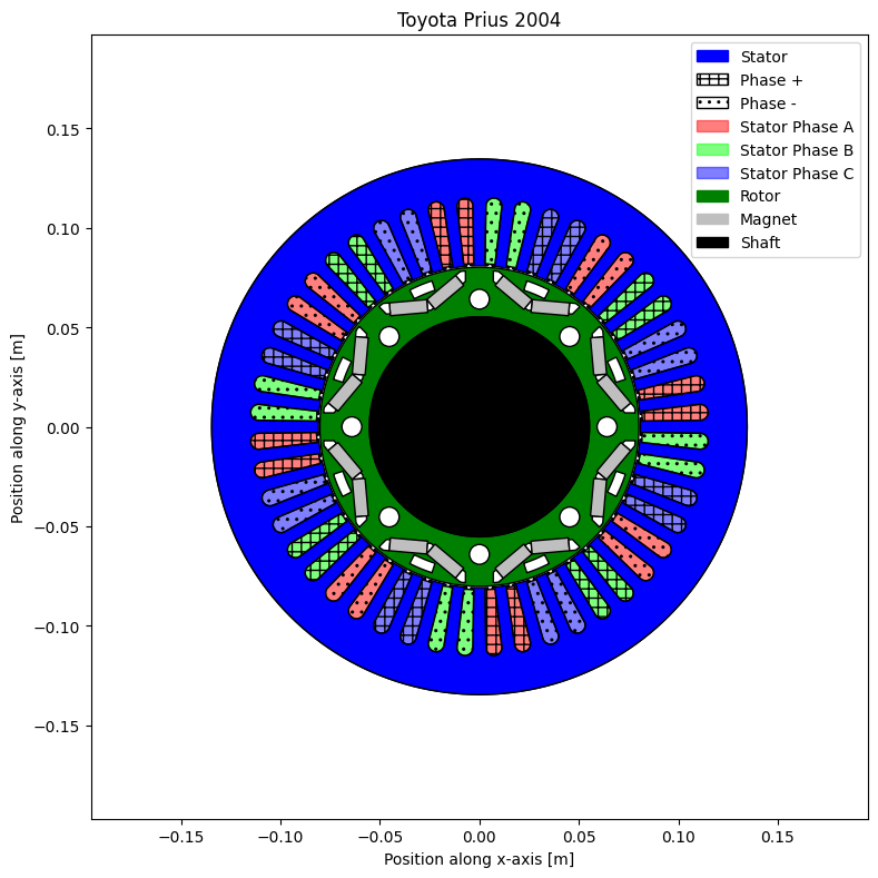
Ventilation duct
[21]:
from pyleecan.Classes.VentilationCirc import VentilationCirc
from pyleecan.Classes.VentilationPolar import VentilationPolar

IPMSM_Prius_2004.rotor.axial_vent = list()
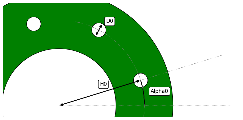
IPMSM_Prius_2004.rotor.axial_vent.append(VentilationCirc(Zh=8, Alpha0=0, D0=10e-3, H0=IPMSM_Prius_2004.rotor.Rext*0.8))
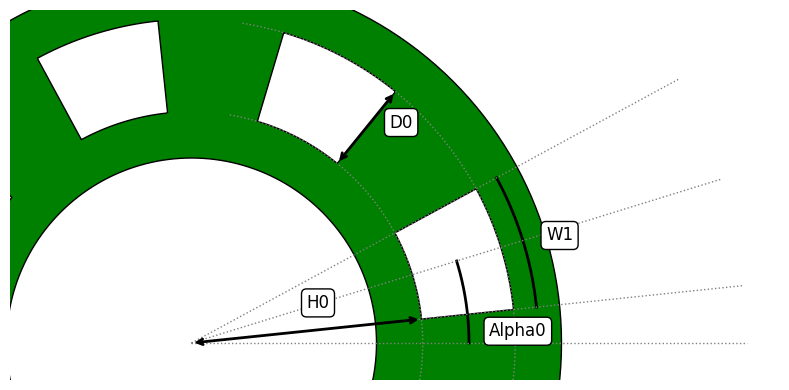
IPMSM_Prius_2004.rotor.axial_vent.append(VentilationPolar(Zh=8, Alpha0=pi/8, W1=pi/20, D0=5e-3, H0=IPMSM_Prius_2004.rotor.Rext*0.9))
fig, ax = IPMSM_Prius_2004.rotor.axial_vent[0].plot_schematics(is_default=True, is_show_fig=False)
fig, ax = IPMSM_Prius_2004.rotor.axial_vent[1].plot_schematics(is_default=True, is_show_fig=False)
fig, ax = IPMSM_Prius_2004.plot(is_show_fig=False)
Notches
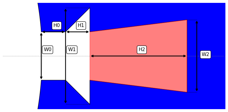
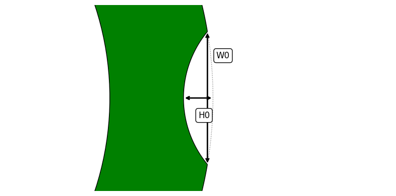
Notches can be added both on rotor and stator and on bore and yoke side. A notch is build with a Slot object which means that the complete Slot library of pyleecan is available for notching without extra work. Notches can be placed one by one (Zs=1) or evenly distributed (Zs>1):
[22]:
from pyleecan.Classes.NotchEvenDist import NotchEvenDist
from pyleecan.Classes.SlotCirc import SlotCirc

slot_s = SlotW10(Zs=12, W0=2.5e-3, W1=5e-3, W2=2.5e-3, H0=2e-3, H1=3e-3, H2=10e-3)
notch_s = NotchEvenDist(notch_shape=slot_s, alpha=0)
fig, ax = slot_s.plot_schematics(is_default=True, is_show_fig=False)

slot_r = SlotCirc(Zs=1, W0=5e-3, H0=5e-3, is_bore=False)  # Single Notch on the rotor yoke
notch_r = NotchEvenDist(notch_shape=slot_r, alpha=pi/16)  # Only one at pi/16
fig, ax = slot_r.plot_schematics(is_default=True, is_show_fig=False)

IPMSM_Prius_2004.stator.notch = [notch_s]
IPMSM_Prius_2004.rotor.notch = [notch_r]
fig, ax = IPMSM_Prius_2004.plot(is_show_fig=False)

Bore shape
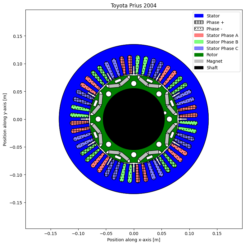
Uneven bore or yoke shape can also be added to any Lamination with:
[23]:
from pyleecan.Classes.BoreFlower import BoreFlower

rotor.bore = BoreFlower(N=8, Rarc=0.06, alpha=pi / 8)
fig, ax = IPMSM_Prius_2004.plot(is_show_fig=False)
[1] Z. Yang, M. Krishnamurthy and I. P. Brown, “Electromagnetic and vibrational characteristic of IPM over full torque-speed range”, 2013 International Electric Machines & Drives Conference, Chicago, IL, 2013, pp. 295-302.
[2] P. Bonneel, J. Le Besnerais, E. Devillers, C. Marinel, and R. Pile, “Design Optimization of Innovative Electrical Machines Topologies Based on Pyleecan Opensource Object-Oriented Software,” in 24th International Conference on Electrical Machines (ICEM), 2020.
[ ]:


